How It Works

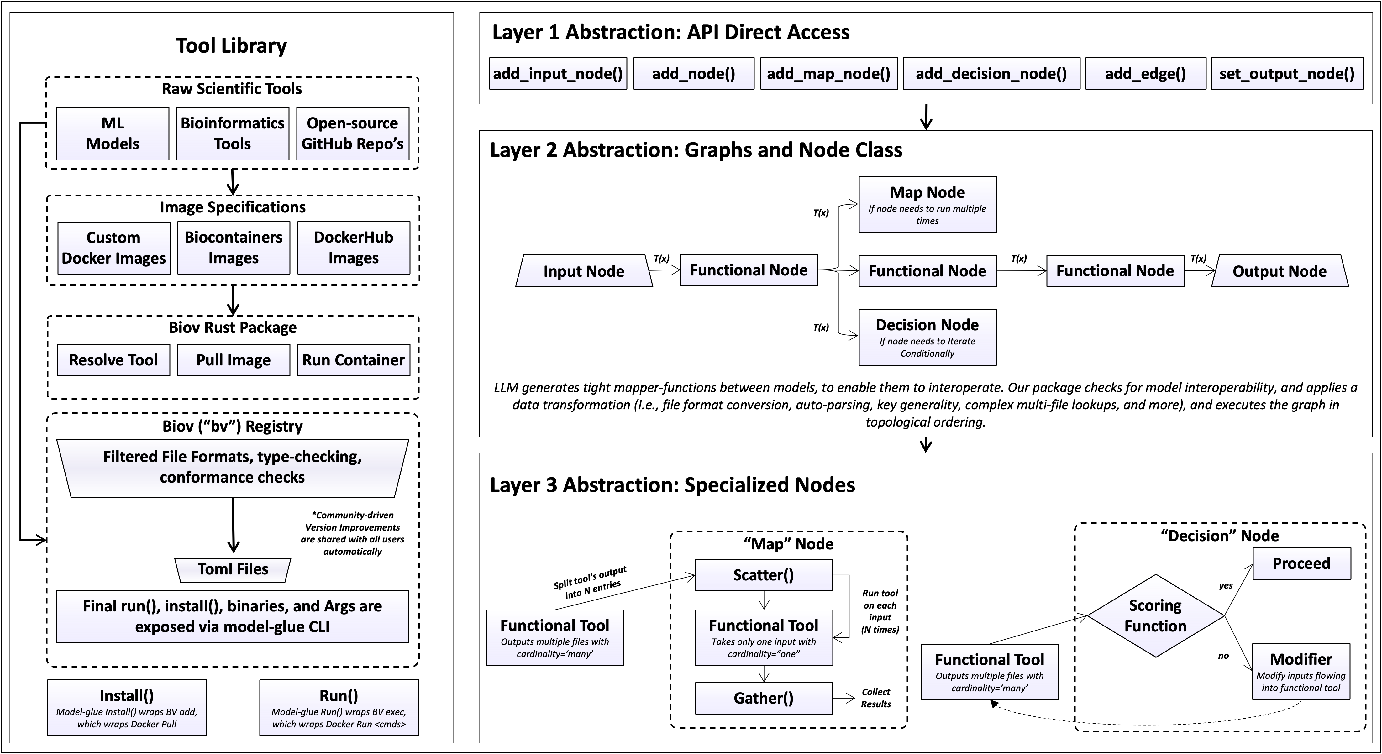
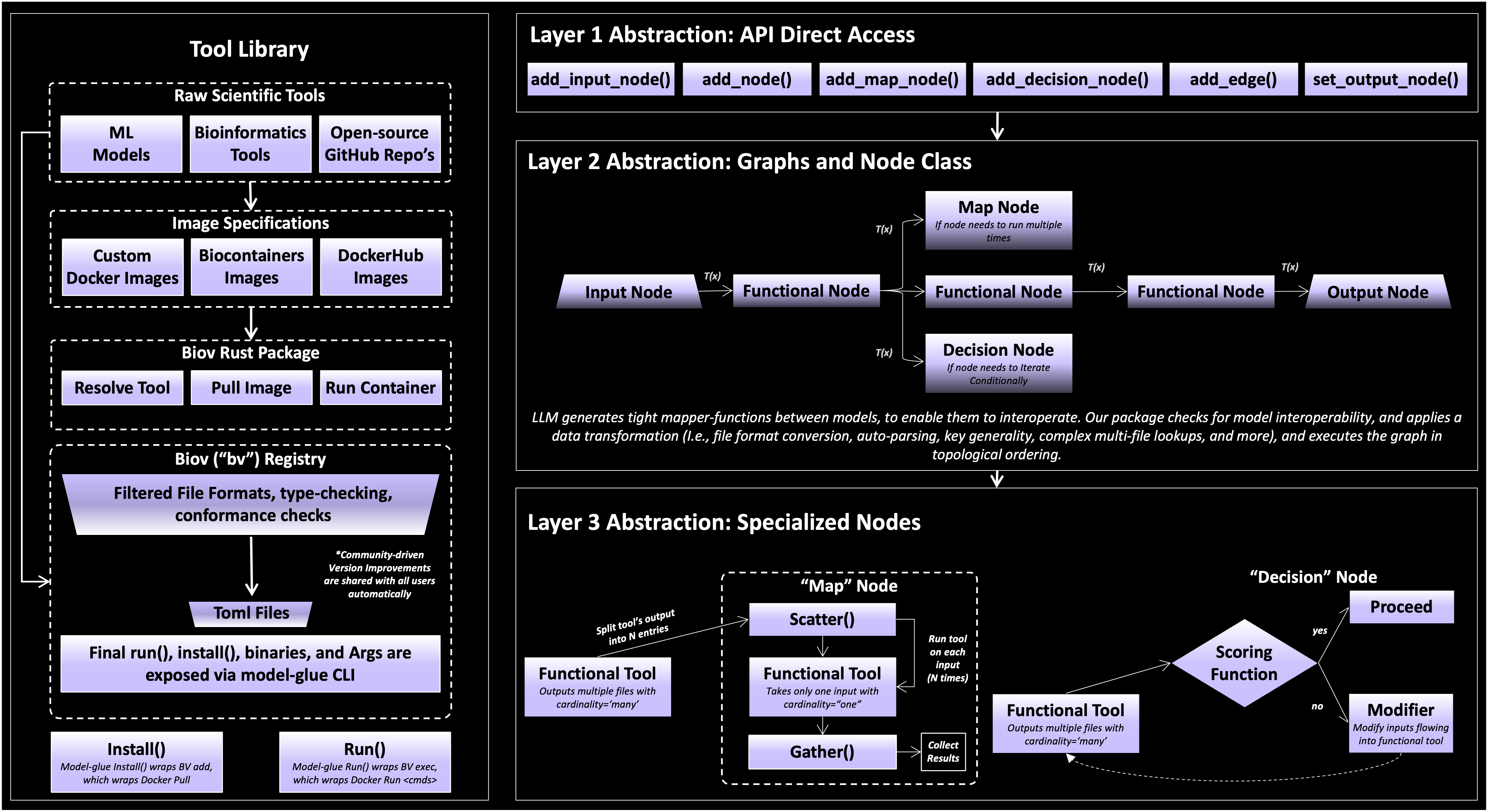
biocomposer decomposes the reasoning required to run a bioinformatics workflow into a stack of abstraction levels, so that at each level only one kind of decision has to be made. Composing tools normally forces the user to reason about everything at once: which tools to chain, how their formats and arguments line up, how to invoke each one, and how to provision its environment. biocomposer separates these concerns into layers, and each layer resolves its own class of decision before delegating the rest downward. The result is that the burden of reasoning about data flow moves smoothly from the user’s intent down to a concrete execution, with no single level holding all of the complexity.

Concretely, a pipeline is expressed against a small Python API; the API operates on a graph of typed nodes; and the nodes are backed by a layer of specializations (connector synthesis, scatter/gather, feedback loops via decision Nodes). Each level is a thin surface over the one beneath it, the user calls add_node(), which resolves a typed tool from the registry, which in turn pulls an image and triggers a container run.

Each layer wraps the one below it: the API surface wraps the graph and node classes, which wrap a layer of specialized helpers; tool installation wraps the registry client, which wraps the container runtime; and the tool library wraps external image sources (BioContainers, Docker Hub).

Pipeline Dataflow

A pipeline is a directed acyclic graph (DAG): tools are nodes and data hand-offs are directed edges.

        flowchart LR
    A(["inputs"]) --> B["align"]
    B --> C["trim"]
    C --> D["fold"]
    D --> E(["result"])
    

The DAG representation gives the system three properties. Dependencies are explicit: an edge A → B declares that B consumes A’s output, and the engine derives run order by traversing the graph backward from the output node, so ordering is never specified by hand. The model generalises past linear chains: fan-out, fan-in, branching, and result sharing are all instances of the same node/edge structure. And it localises data conversion: mapping one tool’s output to another’s input is resolved per edge, against two typed schemas and the actual runtime data, rather than as global script logic.

The API surface

The top layer is a small graph-construction API: add_input_node() for user-supplied values, add_node() for tools, add_edge() to wire them, set_output_node() to mark the result, and execute() to run. Construction is declarative: it records the graph, and no tool runs until execute() is called. These calls are deliberately thin. add_node triggers manifest resolution and image setup beneath it, and execute drives the evaluation described below, so the user never reasons about either.

The graph and node layer

Each node carries the typed input/output schema of its tool’s manifest. The following node types are specified:

• Input nodes hold user files and parameters.

• Tool nodes wrap a single registry tool and run once.

• Gather nodes run a one-input tool once per item of an upstream collection, then gather the results.

• Decision nodes re-run a node with adjusted inputs until a scored condition holds, a feedback loop contained within the node, so the graph as a whole stays acyclic. The score and modifier are each a Python function or a registry tool.

• Subgraphs expose a one-in/one-out pipeline as a single node.

Edges are generated rather than written. Each edge is realised as a connector function from the upstream output schema, the downstream input schema, and a snapshot of the files actually produced at run time; it performs format conversion, field renaming, and selection of the correct file from a directory. Connectors are generated once per edge and cached, so a feedback loop or a wide fan-out reuses a single function (Connectors). When two edges supply the same input key, resolution is deterministic and governed by edge order (Input merging and key clashes). Map, decision, and connector behaviour are themselves a layer of specialized helpers beneath the node classes, the API never exposes them directly.

The tool and container layer

At the base, each tool is a container image paired with a typed manifest. add_node("clustalo") resolves the manifest and pulls the image from DockerHub/Biocontainers/etc. Executing each tool in its own container pins its exact software and versions, making runs reproducible and letting tools with incompatible dependencies coexist in one graph. This layer is itself a wrapper: the tool library sits over external image sources, purpose-built images, BioContainers, or Docker Hub, so adding a tool means writing a manifest over an existing image rather than repackaging it (Tools and the registry, Adding your own tool).

What happens when you call execute()

Building the graph (add_node, add_edge, …) only describes the pipeline. Nothing runs until execute(). At that point biocomposer starts from the final output and works backwards, running each step it depends on. For each step:

        flowchart TD
    U["Upstream step finishes<br/>(produces an output)"] --> C["Connector maps that output<br/>into this step's inputs"]
    C --> S["A fresh sandbox is created"]
    S --> ST["Inputs are copied in;<br/>the command is assembled"]
    ST --> R["The tool runs in its container"]
    R --> H["Outputs are harvested<br/>back out of the sandbox"]
    H --> N["Result passed to the next step"]
    

1. Run upstream first. A step’s inputs come from the steps before it, so those run first (results are reused if a step feeds more than one place).

2. Connect. The connector converts the upstream result into this step’s input dictionary.

3. Sandbox. A temporary working directory (a sandbox) is created. Input files are copied in, output folders are pre-created, and the tool’s command line is assembled from its manifest template (filling in placeholders like {input} and {output}).

4. Execute. The tool runs inside its container, reading and writing only inside the sandbox.

5. Harvest. The files the tool wrote are copied out of the sandbox into a numbered results folder (<tool>_output_1, _2, …), and returned as the step’s output. The sandbox is discarded.

Under the hood: how a tool is actually invoked

For each tool run, biocomposer:

• Installs the tool (bv add + bv sync) the first time it appears, pulling its image. Pulled images are cached on the persistent volume, so later runs restore them locally instead of re-downloading.

• Reads the manifest (bv show --format json) to learn the tool’s inputs, outputs, command, and image.

• Builds a sandbox, a temporary working directory on fast local storage. Input files are copied in flat; output directories are pre-created; the command line is assembled from the manifest’s args_template by filling {slot} placeholders with the staged filenames and scalar values.

• Executes with bv exec inside the tool’s container, with the sandbox as the working directory.

• Harvests the declared outputs back out of the sandbox into a numbered results/ folder, and returns them as the step’s output dictionary.

We also implemented the following: directory-typed outputs are returned as the directory itself (so a connector can look inside it), tools that write stdout are written to .txt format.

Local vs. cloud

The same pipeline script runs in two places (see Installation):

• Locally, using Docker on your machine, fine for lightweight tools.

• On the cloud (Modal), which spins up a remote machine with a GPU, needed for heavy tools like RFdiffusion or ColabFold. biocomposer uploads your script, your inputs/ folder, and itself to a cloud sandbox, runs the pipeline there, and stores results on a persistent cloud volume you can download from.

Because cloud machines are temporary, biocomposer caches downloaded tool images on the persistent volume, so the second run of a large tool doesn’t re-pull the docker image.

Checkpoints

execute() returns the final step’s output as a dictionary of named results, typically paths to the files each tool produced. Every intermediate step’s output is also saved on disk under results/, so nothing is lost between steps.

Note

Tools are cited and used faithfully: each is run as its authors originally presented it, without modifying the original architecture or design choices.